When Good Science Goes Wrong: How Batch Effects Can Obscure Biology

...and how to avoid it

Jul 07, 2025

NOTE: This story is shared with the consent of the researchers who contacted me as a consultant. As requeted by them, details about the experimental design, participant information, metadata and raw and processed data are not disclosed.
This post is written for educational purposes, aimed at wet-lab biologists who want to get the most out of their next -omics experiment. It’s also valuable for bioinformaticians seeking practical advice on how to work around batch effects.

As a bioinformatics consultant, I’m often contacted to advise—or directly assist with—the analysis of various -omics datasets at different stages of a project. One unfortunately recurrent pattern I’ve seen is that researchers who are new to -omics technologies design thoughtful experiments, only to unintentionally undermine the potential insights they might gain. The reason? They sequenced the samples generated in a single experiment across multiple batches. Fortunately, this mistake is as easy to avoid as it is to make.

In this post, I share how you can still extract meaningful insights from your data, using a real-world example I recently worked on. While other blog posts discuss batch effects and how to correct them, I believe they often miss a key point: batch effects should be accounted for at every stage of the data analysis workflow, whenever possible. In this post I will show you how —and why doing so matters. Moreover, I’ll show you that commonly used batch correction software can give a false sense of confidence if used in isolation.

Topics covered in the post:

Batch effects in a nutshell.
A real example of how to work around batch effects.
- Visual assessment of batch effects.
- Accounting for batch effects across stages of the analysis.
Key points and take-home messages.

Batch effects in a nutshell

When a DNA sequence is amplified by a polymerase, there is a chance that the nucleotide bases present in the original template are changed to other bases due to biochemical ‘errors’ of the enzyme. This process is as natural as it is unavoidable.

Importantly, the rate and type of nucleotide changes will vary due to small changes in the conditions in which the polymerase performs the amplification, or due to the nucleotides of the amplified sequence. These natural changes in the original DNA sequences will accumulate across the new sequences as samples go through consecutive amplification cycles.

When sequencing all your samples together, the extent of technical variability they’re subject to is consistent across them. However, when samples generated in just one experiment are sequenced in sub-groups (batches), each batch will acquire a unique, non quantifiable amount of stochastic variation. The introduction of that variability is part of what we call batch effects [1]. Crucially, the technical variations introduced by batch sequencing may obscure the biological patterns that motivated the research in the first place.

Batch effect can distort your data to varying degrees. Imagine a simple experiment in which experimental units (subjects, animals, cells, etc.) are randomly assigned to two conditions (treatment vs control). If all samples from each condition are sequenced in separate batches, the effect of the treatment will be completely confounded by the variability introduced by the sequencing batch. This is one of many problematic scenarios you want to avoid.

Fortunately, you’re now aware of batch effects, and that gives you and edge. However, it’s not always possible to avoid sequencing in batches. By discussing your project in advance with your university’s sequencing facility or a commercial provider, you can define a sequencing strategy that best fit your goals. This ensures you’ll maximize the insights gained from the valuable resources and hard work you’ve invested in your project.

A real example of how to work around batch effects

A few weeks ago, I was contacted by a group of seasoned researchers in the field of diet and brain interactions who wanted to add a microbiome component to their research for the first time. They had collected stool samples from over 230 individuals with different dietary patterns and sent the samples for amplicon (16S rRNA) sequencing. The problem appeared while I was working on the dataset. I noticed something that felt off: a consistent pattern that emerged across all analyses.

I contacted them to set up a meeting and go through details of sampling collection and preparation, thinking that might explain the patterns. Their work was clean. However, near the end of the meeting, they asked me to include some new samples the company had just sent. There was it,. that little something I had been repeatedly seeing in the data. I asked if the samples I worked with had already been sequenced in different batches. Sure they had: four batches, they told me.

Visual assessment of batch effects

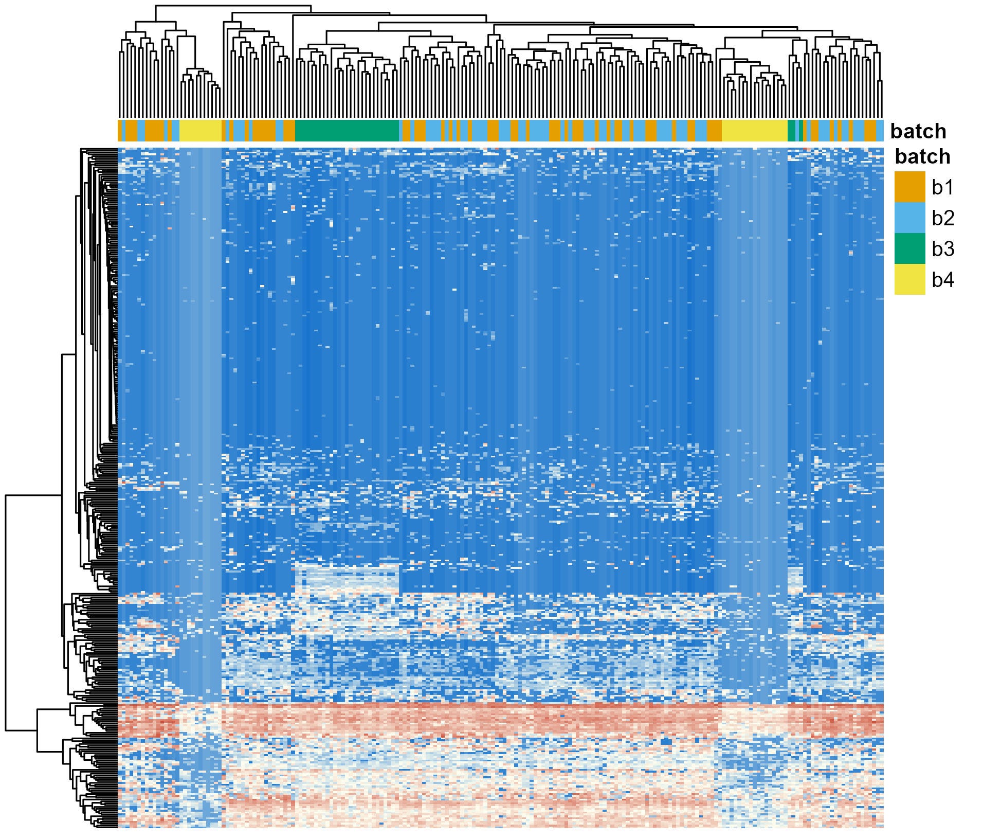
After the meeting, I quickly generated a visualization to asses how prominent the batcheffect was in terms of the variability observed between samples. Heatmaps are a simple but effective way to do this. The idea behind them is that samples are clustered based on how similar they are to one another in terms of the abundances of the different genera. In cases where the batch effect is the strong, samples will cluster by batch regardles of the experimental condition they come from.

I generated the plot (Figure 1). The four sequencing batches are shown in different colors on top row (orange, light blue, green or yellow). The batch effect was clear. Almost all samples from Batch 3 clustered together (i.e., the green block towards the left), and samples from Batch 4 cluster in two distinct groups (each near an edge of the plot). Although the batch effect was cristal clear, I can confidently say I’ve seen worse.

Now, remember: the experimental approach used by these researchers involved clustering subjects due to their dietary patterns. Diet is known to have one of the stronges impact in the stool microbiome composition [2]. Interestingly, regardless of the dietary pattern (not shown, as requested by the authors), the samples clearly cluster due to the batch in which they were sequenced.

**Figure 1: Assessing the effect of batches without any method to account for them.** Heatmap with samples as columns and bacterial genera as rows. On top of the columns, the batches in which samples were sequenced are indicated with colors (organge, blue, green, yellow). The CLR abundance of each genus is shown in shades of blue to red, indicating increased or decreased abundance, respectively. Samples and genera names were removed from the plot as requested by the researchers I collaborated with.

For readers interested in learning more about bioinformatics, I recommend checking out the R package pheatmap for quick generation of heatmaps with clustered samples. I used it to make all plots in this blog post. Heatmaps are based on CLR-transformed abundances, clustered by Euclidian distances. You can find the code in my GitHub repository.

There are several software designed to account for batch effects for virtually every type of -omics data. They share the same goal: to make the biological differences between your experimental groups more prominent by reducing the technical variability introduced by batches. In other (technical) words, they aim to increase the signal-to-noise ratio.

In this post, I show the results of using ComBat [3], a tool originally developed for RNA-seq data but now widely adopted in the microbiome literature.

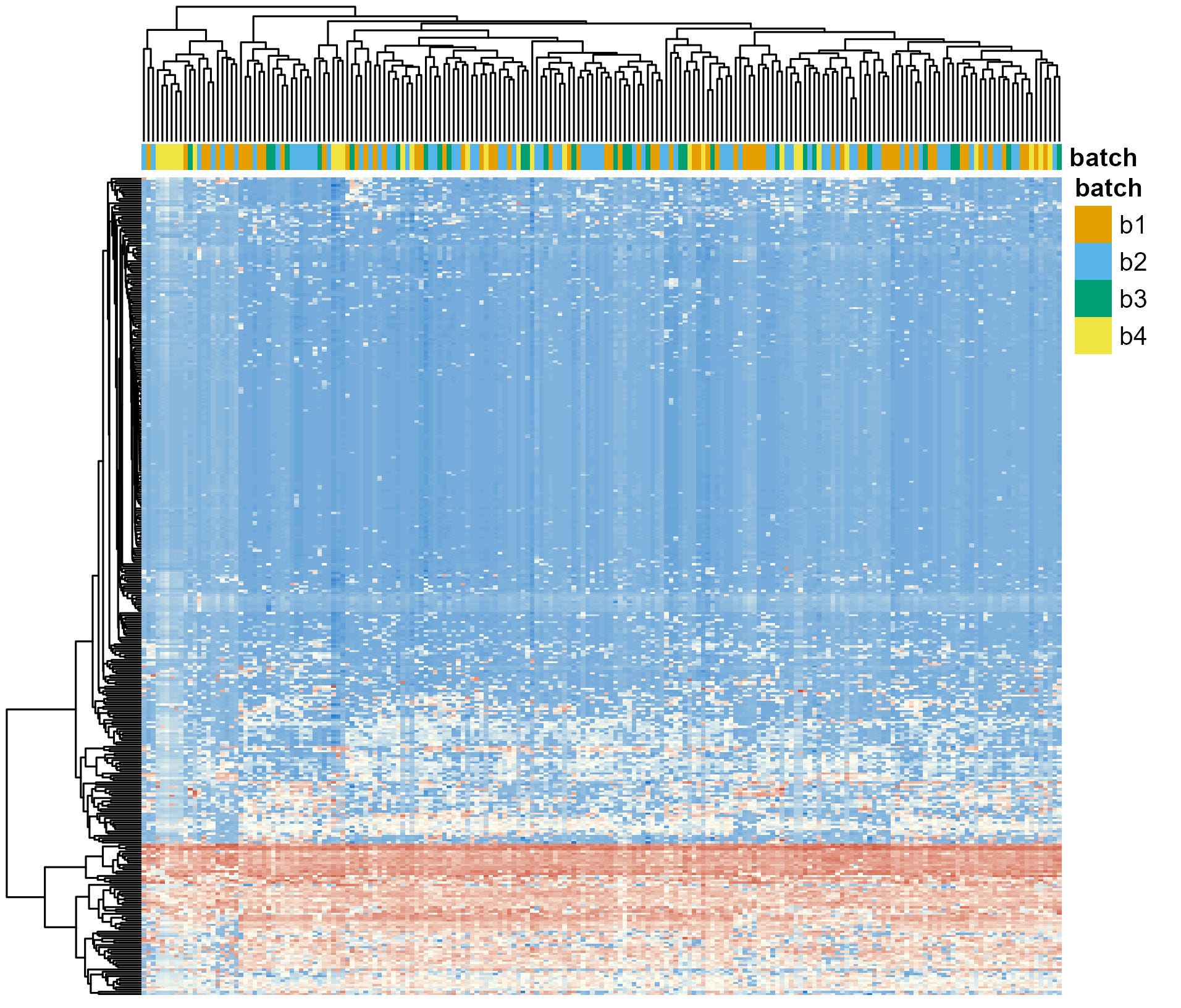
After applying ComBat, the batch effects are drastically reduced (Figure 2). All colors in the top row (batches) are well mixed, indicating that the technical noise has been effectively homogenised across batches.

**Figure 2: Assessing the batch effects after applying the software ComBat trying to remove the batch effect.** Heatmap with samples as columns and bacterial genera as rows. On top of the columns, the batches in which samples were sequenced are indicated with colors (organge, blue, green, yellow). The CLR abundance of each genus is shown in shades of blue to red, indicating increased or decreased abundance, respectively. Samples and genera names were removed from the plot as requested by the researchers I collaborated with.

Accounting for batch effects across stages of the analysis

When I encounter posts discussing batch effects, I often notice they miss a key point: batch effects should be accounted for across all steps of your data analysis workflow. If you see the results above (Figure 2) you might feel confident that your job is done — that batch effects are now controlled and you can actually start your analysis. Unfortunately, batch effects are tougher than that.

If you read the documentation of the DADA2 software, the authors recommend running the software —to learn the error rates of nucleotide substitution— separately for each sequencing run (i.e., batch). As discussed above (See “Batch effects in a nutshell”), small differences in the intial sequencing conditions can impact the rate at which nucleotides in your sequences are substituted by others, a process that is natural and unavoidable.

To address this, authors of DADA2 [4] developed an algorithm designed to discriminate between nucleotide changes caused by technical variation and those resulting from true biological (evolutionary) process. Therefore, using their algorithm independently for each batch is a crucial step, as the error rates will be batch-specific.

Importantly, every -omics technologies has its own ways in which batch effects can be addressed throughout the different stages of analysis. Here I focus only on 16S rRNA amplicon sequencing, as that was the technology used by the researchers who contacted me.

So, I restarted the analysis of the raw amplicon sequencing data. This time, I used a for loop to run the DADA2 workflow for each batch separately, up to the point were the ASV-level count tables were generated for each batch (See “Infer Sequence Variants”). Then, I used another script to merge all those count tables and complete the classic DADA2 workflow (See “Merge Runs, Remove Chimeras, Assign Taxonomy”). Results are shown in Figure 3.

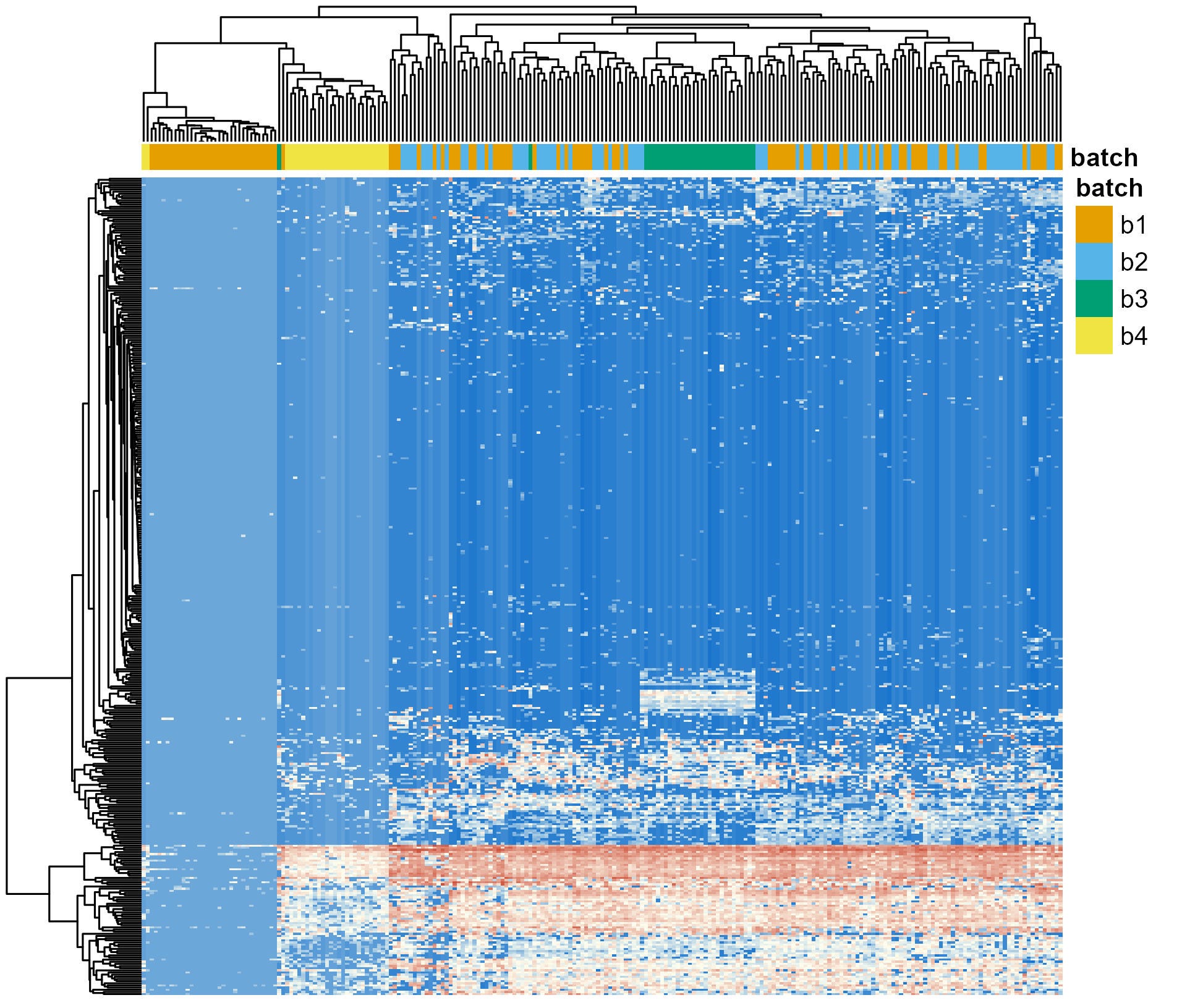
**Figure 3: Assessing the batch effects after learning error rates with DADA2 for each batch independently.** Heatmap with samples as columns and bacterial genera as rows. On top of the columns, the batches in which samples were sequenced are indicated with colors (organge, blue, green, yellow). The CLR abundance of each genus is shown in shades of blue to red, indicating increased or decreased abundance, respectively. Samples and genera names were removed from the plot as requested by the researchers I collaborated with.

You could argue that, this time, the distorting effects of batches are worse than before. Batch 4 (yellow) now clusters almost entirely together, a significant number of samples from Batch 1 are clustering as well. This constrasts with the more homogeneous distribution I showed you in Figure 1.

However, I’d argue that what we’re seeing now is a more accurate assessment of the extent to which batch effects can distort the data. You’re not convinced? Let me give you more context and show you a new plot.

After applying the first batch correction step—learning error rates for each batch independently—I followed up with a second: applying ComBat (Figure 4). The results are similar to what I showed you before (Figure 2). Samples don’t cluster by batch anymore. Except for all those samples in batch 1 that still do.

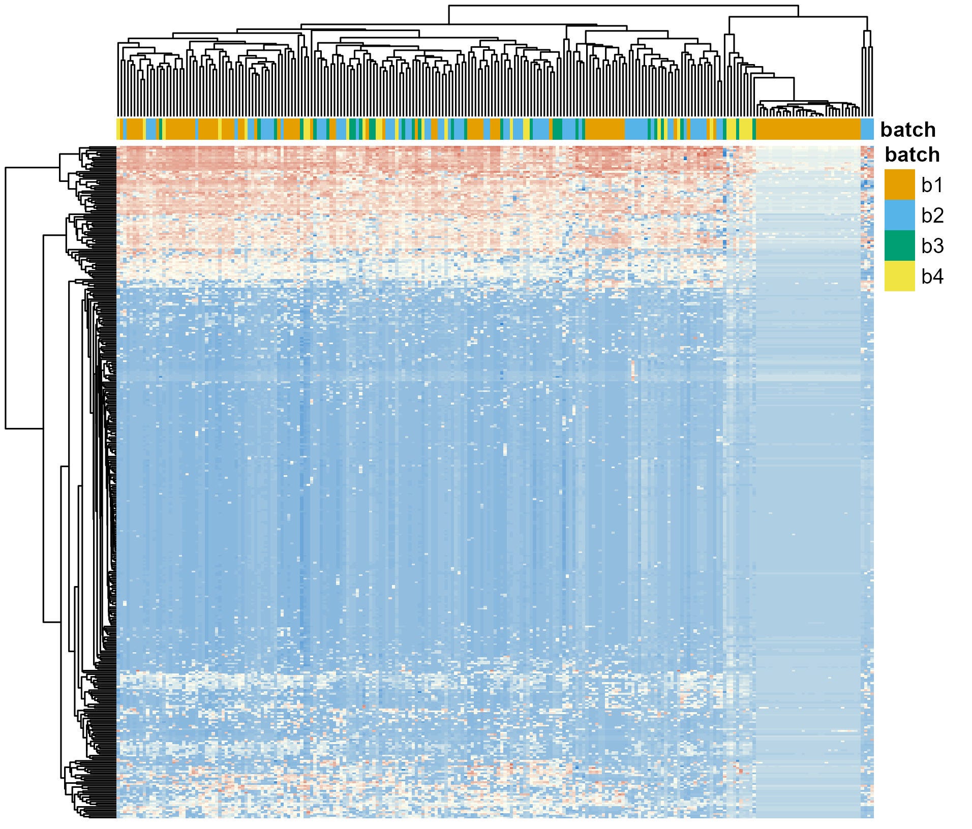
**Figure 4: Assessing the batch effects after learning error rates with DADA2 for each batch independently and applying ComBat.** Heatmap with samples as columns and bacterial genera as rows. On top of the columns, the batches in which samples were sequenced are indicated with colors (organge, blue, green, yellow). The CLR abundance of each genus is shown in shades of blue to red, indicating increased or decreased abundance, respectively. Samples and genera names were removed from the plot as requested by the researchers I collaborated with.

With this new information I reached back again to the researchers. Instead of telling them exactly what happened, I just asked them to corroborate that the information they gave me about the list of samples included in each batch was accurate. Surprisingly, they had made a mistake in the information. They sequenced their samples in 5 batches and two of them were coded as “Batch 1” in the file they sent me.

On a side note, in a later conversations they told me that Batch 3 was actually sequenced with a different Illumina technology. Interestingly, ComBat had no issue accounting for that when attempting to remove batch effects (Figures 2 and 4). Of course, sequencing with different technologies is not a recommended strategy.

In the following sessions with those researchers, we will continue with the analysis of their biological hypotheses. Whether they decide to keep those samples in the analysis or not is not clear now. Regardless of their decision, the effects of batches need to still be accounted for in the following analyses. For instance, by including that information as covariates when building the statistical models used to test their biological hypotheses.

Key points and take home messages

TL;DR: I shared my experience consulting for a group of scientists who, although experts in their field, were starting their first -omics experiment. They sequenced their samples in batches, thus introducing technical variation that can potentially obscure biological signals they were investigating. In this post, we discussed what batch effects are, why we want to avoid generating them, and how we can account for them in our bioinformatics analysis. Moreover, I showed you that common software used in batch effect correction can give a false sense of confidence if used in isolation.

Take-home messages:

Avoid generating batches whenever possible. If batches are unavoidable, talk to the team or commercial provider doing the sequencing of your samples, and then to your bioinformatician(s).
Any -omics technology is subject to batch effects. I just used this amplicon sequencing project as an example.
Approaches to account for batch effects should be used across all stages of the analysis. Failing to do so may lead to a false sense of confidence. For instace, starting by building the models of error rates in DADA2 separately for each batch, then using software to increase the signal to noise ration (ComBat or others), and then using the information about from what batch samples come from when building the statistical models used to test your biological hypotheses.

Leek, J., Scharpf, R., Bravo, H. et al. Tackling the widespread and critical impact of batch effects in high-throughput data. Nat Rev Genet 11, 733–739 (2010). https://doi.org/10.1038/nrg2825

The Middle Author Bioinformatician

Discussion about this post